
Tutorial
This tutorial shows how to use the ALCF to process ceilometer observations, simulate lidar from model output and compare the two. As an example, we will use 24 hours of Lufft CHM 15k ceilometer observations at the Birdlings Flat site in Canterbury, New Zeland on 4 July 2016, and the corresponding Antarctic Mesoscale Prediction System (AMPS) numerical weather prediction (NWP) model and MERRA-2 renalaysis output. To start, download the dataset archive alcf-tutorial-datasets.zip (4.3 GB).
Note: Normally, you would want to compare more than 24 hours of measurements, such as one month or one year. This tutorial uses 24 hours of data due to the large size of the datasets.
Processing with the ALCF can be done in two modes: automatic and manual. The automatic mode is easier and is convered in this tutorial. Both automatic and manual processing are equivalent, but manual processing gives you a better understanding of the processing steps and can be more useful if anything goes wrong during the processing. Please see the documentation on how to perform manual processing.
Preparation
First, make sure that you have installed the ALCF following the installation
instructions, and the you can run alcf in the
terminal. Extract the archive alcf-tutorial-datasets.tar in your working
directory:
unzip alcf-tutorial-datasets.zip
cd alcf-tutorial-datasets
Datasets
The contents of the dataset archive are:
raw: raw ceilometer and model filesraw/amps: AMPS NWP model dataraw/chm15k: Lufft CHM 15k dataraw/merra2: MERRA-2 reanalysis data
The data files are stored in the NetCDF format and can be previewed with Panoply, HDFView, ncdump or ds.
Automatic processing
Observations
To process the observations use the following command:
mkdir -p processed # Create directory "processed".
alcf auto lidar chm15k raw/chm15k processed/chm15k
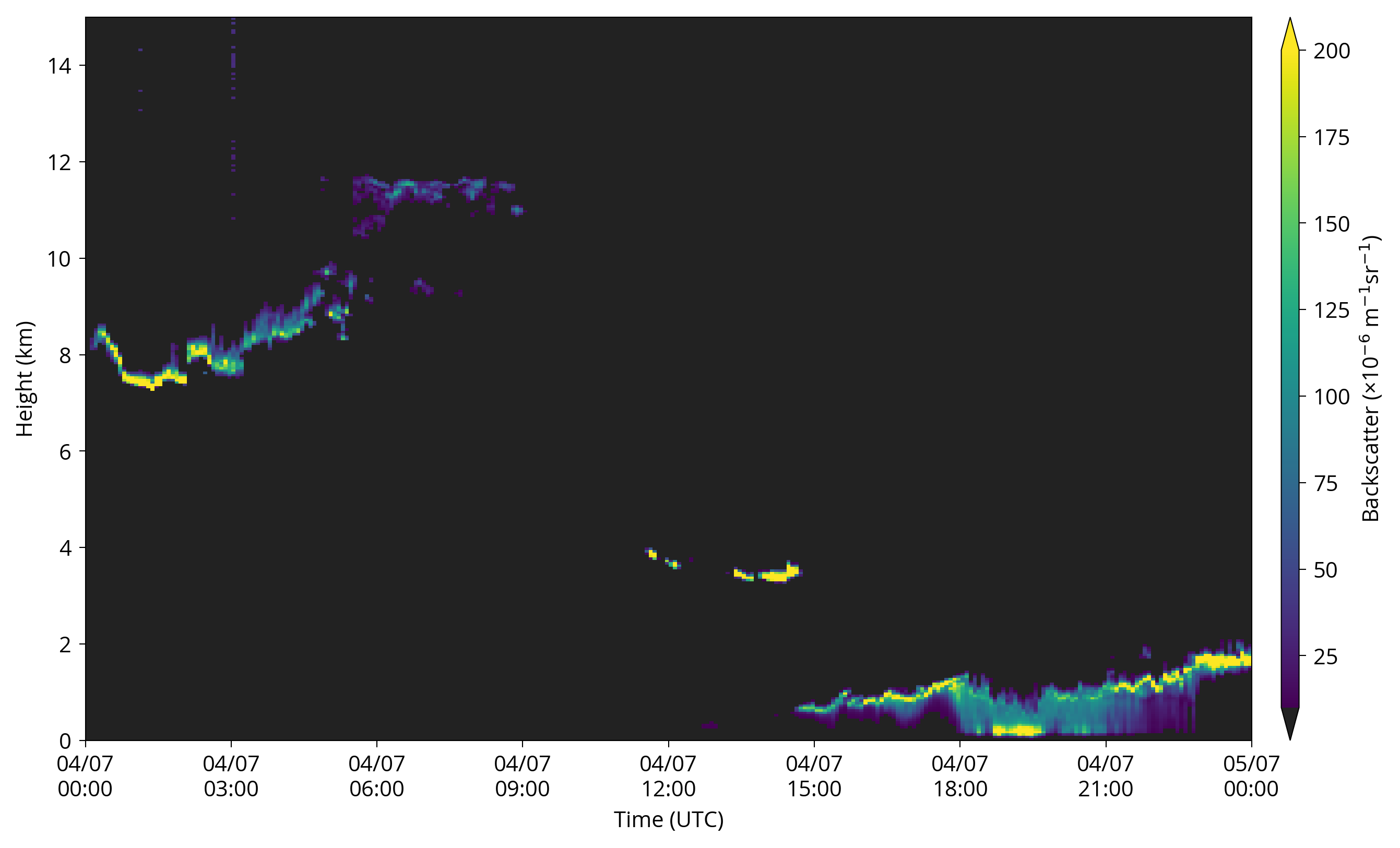
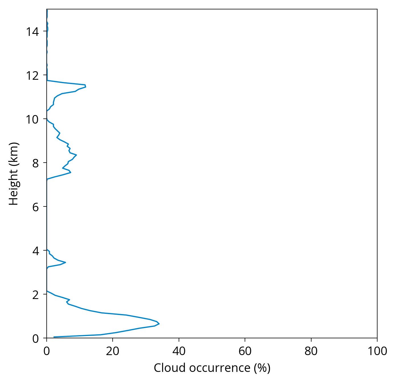
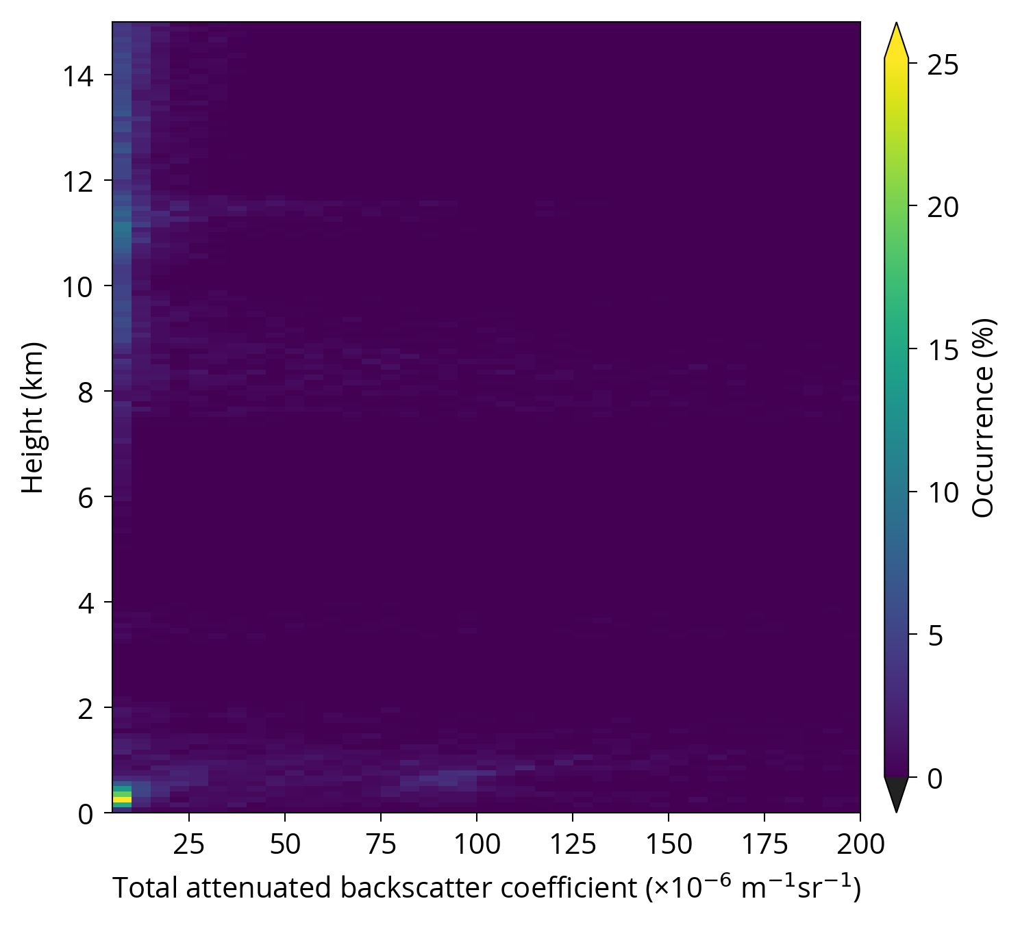
This command will resample the lidar data, remove noise, detect clouds,
calculate statistics, and plot the lidar backscatter, backscatter histogram
and cloud occurrence as a function of height. The output will
be stored in processed/chm15k:
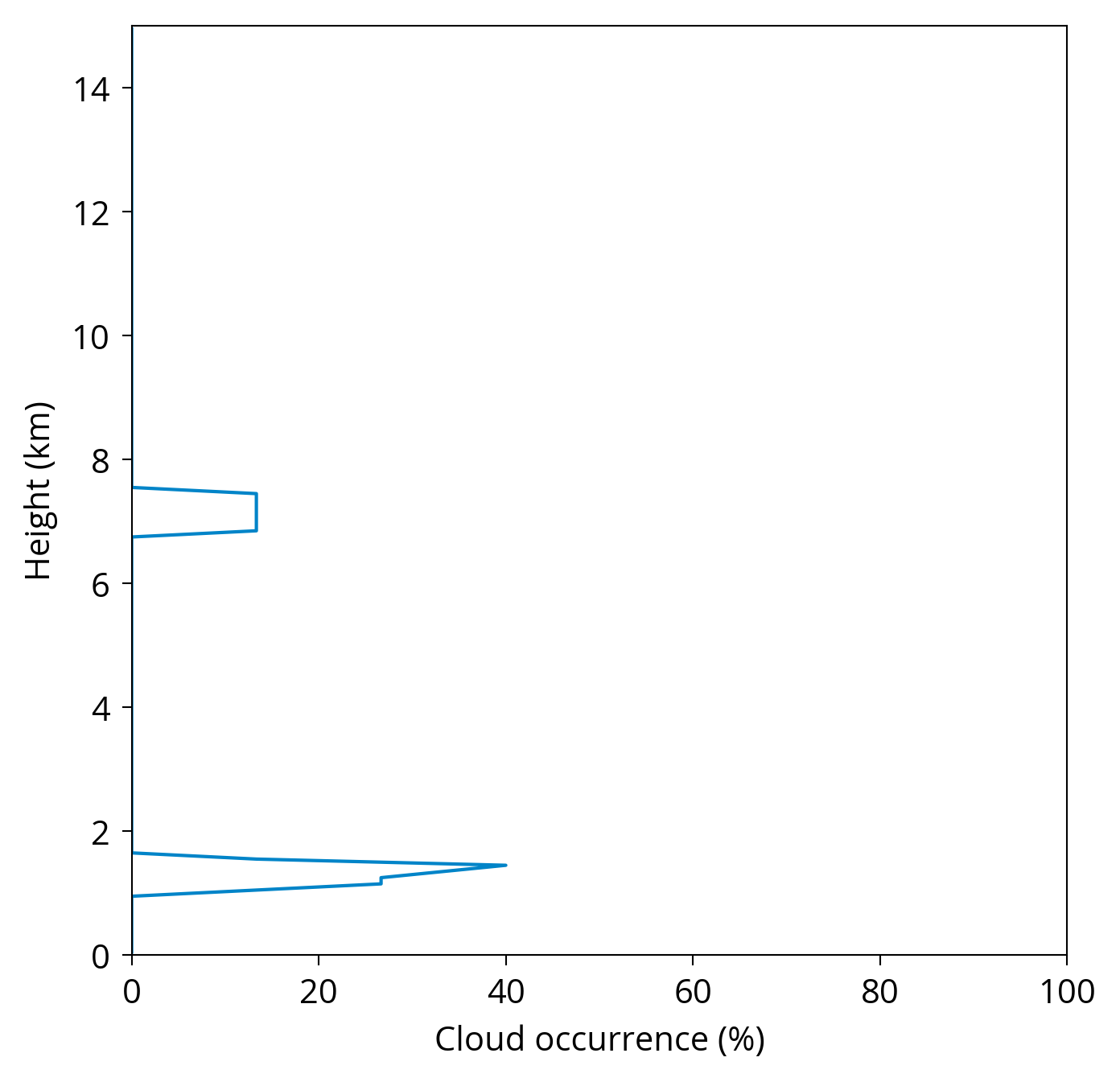
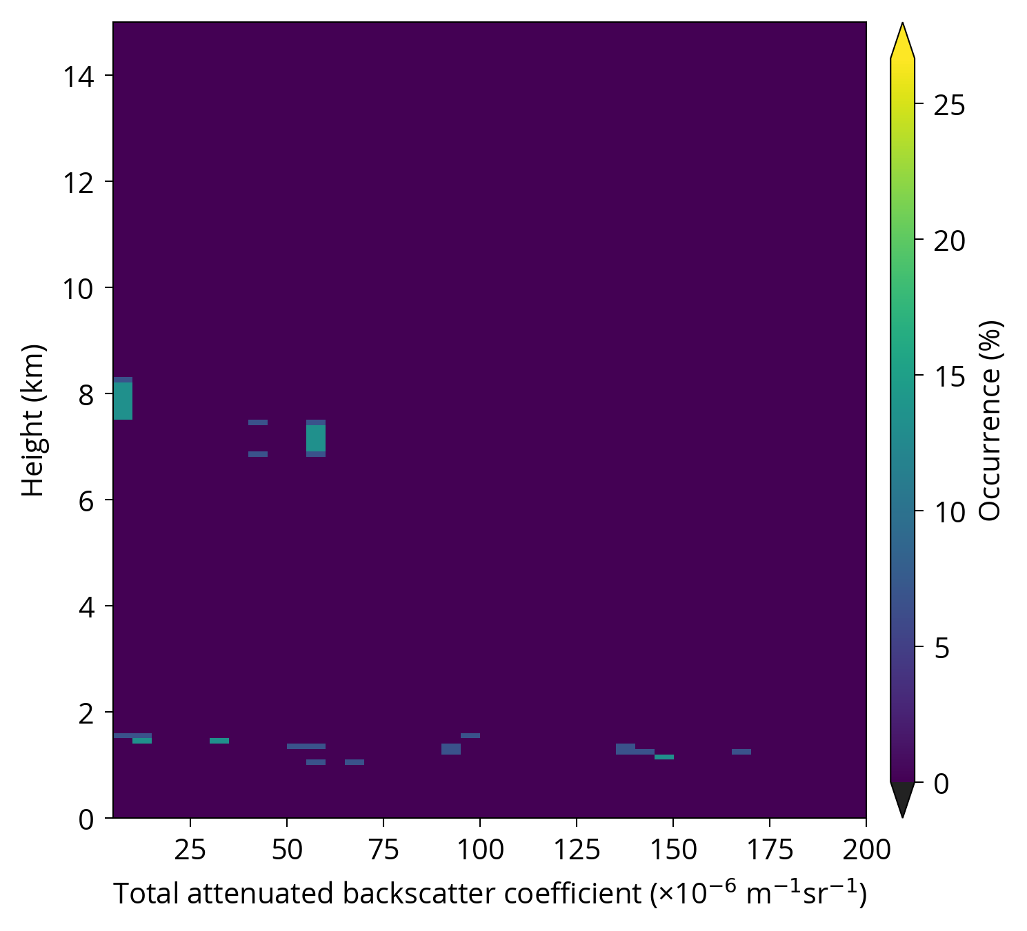
lidar: processed lidar data as daily files (NetCDF)plot: plotsplot/backscatter: daily backscatter profile plotsplot/backscatter_hist.png: plot of backscatter histogramplot/cloud_occurrence.png: plot of cloud occurrence histogram as a function of heightstats: statisticsstats/all.nc: statistics (NetCDF)
Figure 1 shows the Lufft CHM 15k plots. See the ALCF output for description of the NetCDF files.
If the input directory with lidar data files contains subdirectories, add the
-r option at the end of the alcf auto command to process all subdirectorie
recursively in alphabetical order.
Some lidars (Vaisala CL31, CL51) produce data files in a custom data format
which has to be converted to NetCDF before using alcf auto or alcf lidar.
Use the command alcf convert cl51 <input> <output> to convert the DAT files
to NetCDF, where input is an input directory with DAT files and output
is an output directory where the NetCDF files are to be written. The -r
option can be used to process the input directory recursively.
Model
To process MERRA-2 model data use the following command:
mkdir -p processed # Create directory "processed".
alcf auto model merra2 chm15k raw/merra2 processed/merra2 \
    point: { 172.686 -43.821 } time: { 2016-07-04T00:00 2016-07-05T00:00 }
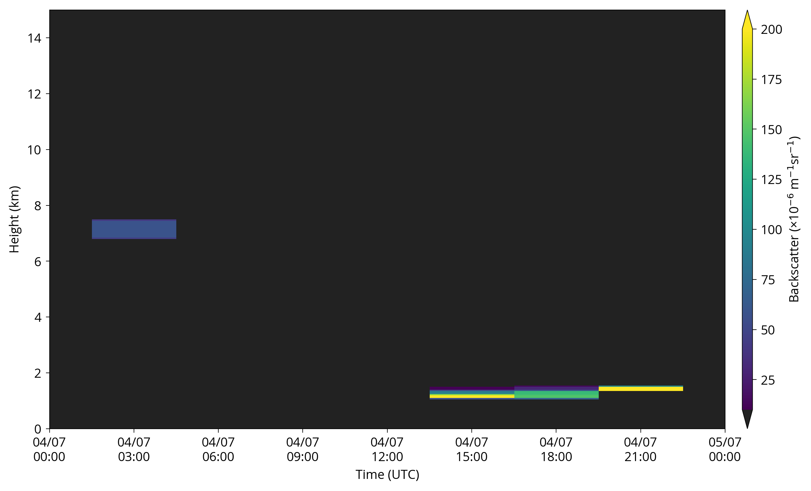
The command will extract a “curtain” of data along the give point and time
period, run the lidar simulator on the extracted data,
simulating the Lufft CHM 15k instrument, and run the same processing steps as
alcf auto lidar on the observational data above.
The output will be stored in processed/merra2:
model: extracted model data along the geographical point and time period (NetCDF)simulate: simulated lidar backscatter (NetCDF)lidar: processed lidar data as daily files (NetCDF)plot: plotsplot/backscatter: daily backscatter profile plotsplot/backscatter_hist.png: plot of backscatter histogramplot/cloud_occurrence.png: plot of cloud occurrence histogram as a function of heightstats: statisticsstats/all.nc: statistics (NetCDF)
Figure 2 shows the MERRA-2 plots. See the ALCF output for description of the NetCDF files.
If the input directory with model data files contains subdirectories, add the
-r option at the end of the alcf auto command to process all subdirectorie
recursively in alphabetical order.
Some model (JRA-55) produce data files in a custom data format which has to be
converted to NetCDF before using alcf auto or alcf model. Use the command
alcf convert jra55 <input> <output> to convert the GRIB files to NetCDF,
where input is an input directory with GRIB files and output is an output
directory where the NetCDF files are to be written. The -r option can be used
to process the input directory recursively.
Conclusion
This tutorial introduced how to use the ALCF to process 24 hours of data collected by the Lufft CHM 15k ceilometer and the corresponding data from the MERRA-2 reanalysis. The ALCF supports more advanced options described in the documentation. For support please see the support page.